Attention on the Simplex

Introduction

From language models to vision systems, transformers have took the scene as a all-in-one architechtures, and at their core lies the attention mechanism. We often visualize attention as heatmaps: grids of numbers showing how much each token “looks at” every other token. But these heatmaps, while useful, hide a rich geometric structure.

What if we could see attention patterns as shapes? As points, lines, and volumes inside a well-known geometric object?

It turns out we can. Each row of an attention matrix is a probability distribution, and probability distributions live on a beautiful geometric object called a simplex. By plotting attention rows on the simplex, we can literally see the difference between a “sink head” (all tokens staring at one place), a “copying head” (each token looking at its predecessor), and a “mixing head” (attention spread across everything).

Of course, there is a catch: this visualization only works in low dimensions — up to $4 \times 4$ attention matrices, which map onto a tetrahedron we can plot in 3D. Real transformers operate in much higher dimensions. But even in this toy setting, the geometric view offers intuitions that transfer: rank constraints become visible as dimensional collapses, diversity becomes volume, and selectivity becomes proximity to vertices.

Let us take this walk from definitions to pictures.

Step 1: Simplices and Attention

The Simplex

An $(n{-}1)$-simplex $\Delta^{n-1}$ is the set of all probability distributions over $n$ outcomes:

\[\Delta^{n-1} = \left\{ (p_1, \ldots, p_n) \in \mathbb{R}^n \;\middle|\; p_i \geq 0, \;\sum_{i=1}^n p_i = 1 \right\}\]

For small $n$:

$n = 2$: a line segment (between “all on token 1” and “all on token 2”)
$n = 3$: a triangle (the 2-simplex)
$n = 4$: a tetrahedron (the 3-simplex).

The vertices of the simplex are the “pure” distributions: $e_1 = (1, 0, 0, 0)$, $e_2 = (0, 1, 0, 0)$, etc. The center $(1/n, \ldots, 1/n)$ is the uniform distribution.

Attention

In a transformer, given queries $Q$, keys $K$, and values $V$, the attention mechanism computes:

\[A = \text{softmax}\!\left(\frac{QK^\top}{\sqrt{d_k}}\right)\]

The result $A$ is an $n \times n$ row-stochastic matrix: every row sums to 1, every entry is non-negative. Each row $a_i$ tells us how token $i$ distributes its attention over all $n$ tokens.

Each row $a_i$ is therefore a point on the $(n{-}1)$-simplex $\Delta^{n-1}$.

Step 2: Why Attention Lives on the Simplex

This is the key insight: an $n \times n$ attention matrix $A$ places $n$ points on the $(n{-}1)$-simplex. Row $i$ of $A$ is the point in $\Delta^{n-1}$ representing the attention distribution of token $i$.

The convex hull of these $n$ points, the smallest convex shape containing them. is what we call the row polytope of $A$. The geometry of this polytope encodes properties of the attention pattern:

Geometric property	Attention interpretation
Points clustered together	Rows are similar — tokens attend similarly (low diversity)
Points near vertices	Rows are peaked — tokens attend selectively (high selectivity)
Points near the center	Rows are diffuse — attention is spread out (high entropy)
Polytope has large volume	Rows are diverse — different tokens attend very differently
Polytope is flat (low-dimensional)	The matrix has low rank — a few “prototypes” generate all rows

The rank of the attention matrix constrains the dimension of the polytope:

Rank 1: all rows are identical → the polytope is a single point
Rank 2: rows lie on a line within the simplex
Rank 3: rows lie on a plane (a 2D surface within the simplex)
Rank $n$: rows can span the full simplex — the polytope is a genuine $(n{-}1)$-dimensional solid

In general, the row polytope lives in a $(r{-}1)$-dimensional affine subspace, where $r = \text{rank}(A)$. This is because rank-$r$ means the rows live in an $r$-dimensional linear subspace, and intersecting that with the simplex (the constraint $\sum a_i = 1$) removes one degree of freedom.

Step 3: Five Archetypes on the 3-Simplex

We now consider $4 \times 4$ attention matrices, the sweet spot where we can still visualize things in 3D (the 3-simplex is a tetrahedron). We pick five archetypal patterns that appear in real transformer heads:

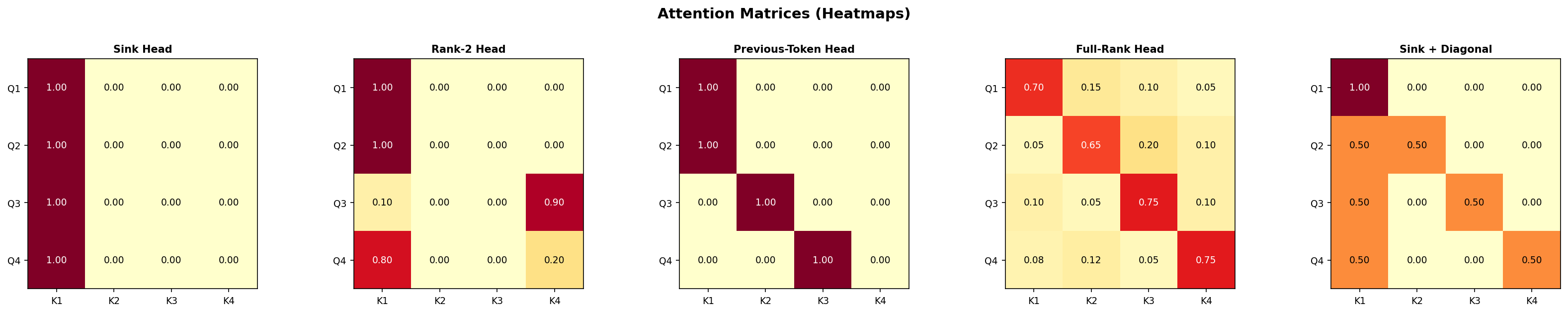
Attention heatmaps for the five archetypes

1. The Sink Head

\[A_{\text{sink}} = \begin{pmatrix} 1 & 0 & 0 & 0 \\ 1 & 0 & 0 & 0 \\ 1 & 0 & 0 & 0 \\ 1 & 0 & 0 & 0 \end{pmatrix}\]

Every token sends all its attention to token 1 (the “sink” or “BOS” token). All four rows are the same point: the vertex $e_1$. The polytope is a single point. Rank = 1.

This is the degenerate extreme: maximum selectivity, zero diversity. In practice, some attention heads in language models do exactly this: they learn to “park” attention on a designated token when there is nothing useful to attend to. These are sometimes called attention sinks or null heads.

2. The Rank-2 Head

\[A_{\text{rank2}} = \begin{pmatrix} 1 & 0 & 0 & 0 \\ 1 & 0 & 0 & 0 \\ 0.1 & 0 & 0 & 0.9 \\ 0.8 & 0 & 0 & 0.2 \end{pmatrix}\]

All rows live in the span of $e_1$ and $e_4$ — columns 2 and 3 are identically zero. The polytope is a line segment along the edge connecting $e_1$ to $e_4$. Rank = 2.

This is the simplest non-trivial case: the head can only mix between two “prototype” attention targets (token 1 and token 4). Two rows are pinned at $e_1$, while the others slide along the $e_1$–$e_4$ edge. On the simplex, all rows are collinear — the row polytope is one-dimensional.

Rank-2 attention arises when the query-key interaction effectively reduces to a single discriminating direction. It is a common regime in early layers or in heads that specialize in binary decisions (attend to this token or that one).

3. The Previous-Token Head

\[A_{\text{prev}} = \begin{pmatrix} 1 & 0 & 0 & 0 \\ 1 & 0 & 0 & 0 \\ 0 & 1 & 0 & 0 \\ 0 & 0 & 1 & 0 \end{pmatrix}\]

Each token attends to the token before it (with the first token attending to itself, and assuming a causal mask). The rows are $e_1, e_1, e_2, e_3$ — three distinct vertices of the tetrahedron. The polytope is a triangle (a 2D face of the tetrahedron). Rank = 3.

This pattern implements a shift operation: the output at position $i$ copies the value from position $i{-}1$. It is highly selective (each row is a vertex = a delta distribution) and highly diverse (rows point in completely different directions). Previous-token heads are among the most commonly identified “induction” circuit components.

4. The Full-Rank Head

\[A_{\text{full}} = \begin{pmatrix} 0.70 & 0.10 & 0.10 & 0.10 \\ 0.10 & 0.70 & 0.10 & 0.10 \\ 0.10 & 0.10 & 0.70 & 0.10 \\ 0.10 & 0.10 & 0.10 & 0.70 \end{pmatrix}\]

Each token mostly attends to itself, with some residual attention spread uniformly. The four rows form a tetrahedron inside the simplex: the polytope is a scaled-down copy of the full simplex, centered but shifted toward the vertices. Rank = 4 (full rank, generically as we perturb from identity). Actually this specific matrix has rank 2 since $A = 0.1 \cdot \mathbf{1}\mathbf{1}^\top + 0.6 \cdot I$ but let us use a less symmetric version:

\[A_{\text{full}} = \begin{pmatrix} 0.70 & 0.15 & 0.10 & 0.05 \\ 0.05 & 0.65 & 0.20 & 0.10 \\ 0.10 & 0.05 & 0.75 & 0.10 \\ 0.08 & 0.12 & 0.05 & 0.75 \end{pmatrix}\]

Now the rows genuinely span a 3D region inside the tetrahedron — the polytope has volume. This represents an attention head with maximum expressive freedom: every token has a distinct, non-degenerate attention pattern.

5. The Sink + Diagonal Head

\[A_{\text{sink+diag}} = \begin{pmatrix} 1 & 0 & 0 & 0 \\ 0.50 & 0.50 & 0 & 0 \\ 0.50 & 0 & 0.50 & 0 \\ 0.50 & 0 & 0 & 0.50 \end{pmatrix}\]

Token 1 is a pure sink. Tokens 2–4 split their attention between the sink and themselves. The rows form a pattern: $e_1$ is at a vertex, and the other three rows are midpoints of edges emanating from $e_1$. The polytope is a triangle (2D), but it is “anchored” at the sink vertex.

This is a common pattern in early layers of transformers: a combination of positional (self-attention on the diagonal) and a learned bias toward a sink token. It has rank 4 (each row is distinct), but its geometry is constrained — the polytope is flat because rows 2–4 are all convex combinations of $e_1$ and one vertex.

Seeing All Five on the Simplex

The interactive 3D visualizations below (generated with Plotly — drag to rotate, scroll to zoom, hover for details) show each polytope inside the tetrahedron:

Explore each archetype individually:

Polytopes and Geometric Quantities

Once we see attention as polytopes on the simplex, we can measure their geometry:

Volume (or Area, or Length)

The $(r{-}1)$-dimensional volume of the row polytope quantifies diversity: how different are the attention patterns of different tokens?

Volume = 0: all rows are identical (rank 1) or collinear (rank 2 with zero length only if degenerate)
Small volume: rows are similar — the head computes similar functions for all tokens
Large volume: rows are diverse — the head differentiates strongly between tokens

Distance to Vertices

The average distance of the rows to the nearest vertex measures selectivity:

Close to vertices: peaked distributions (low entropy, sharp attention)
Close to center: diffuse distributions (high entropy, spread attention)

Centroid Position

Where the centroid (average row) falls in the simplex tells us about bias: does the head, on average, favor certain tokens?

Step 4: Connections to Information Geometry

The simplex is not just a flat triangular surface — it carries a natural curved geometry given by information theory.

The Fisher-Rao Metric

The Fisher-Rao metric endows the simplex with a Riemannian structure where the distance between two distributions $p, q \in \Delta^{n-1}$ is:

\[d_{FR}(p, q) = 2 \arccos\!\left(\sum_{i=1}^n \sqrt{p_i \, q_i}\right)\]

This is the geodesic distance on the “statistical manifold.” Under this metric, the simplex is (a piece of) a sphere: the map $p \mapsto 2\sqrt{p}$ sends the simplex to the positive orthant of the unit sphere.

What does this mean for attention? The Fisher-Rao distance between two rows of the attention matrix measures how “informationally different” the two attention patterns are — not in the flat Euclidean sense, but in a way that respects the probabilistic nature of the distributions.

Near the vertices (peaked distributions), the Fisher-Rao metric “stretches” — small changes in attention weights correspond to large informational differences. Near the center (uniform distribution), the metric “compresses” — the same numerical change matters less. This is exactly the right notion: changing attention from 0.01 to 0.02 (doubling!) is more significant than changing from 0.50 to 0.51.

Uncertainty and Entropy

The entropy of a row $H(a_i) = -\sum_j a_{ij} \log a_{ij}$ measures uncertainty — how uncertain is token $i$ about where to attend?

On the simplex, entropy defines a “height function”: the center has maximum entropy ($\log n$), and the vertices have minimum entropy (0). Lines of constant entropy are “level sets” — curves on the simplex where all distributions have the same uncertainty.

There is a beautiful uncertainty principle at play: a row cannot be simultaneously close to two different vertices. If $a_i$ is close to $e_j$ (high attention on token $j$), it must be far from all other vertices. The simplex geometry enforces this tradeoff between attending to one thing vs. spreading attention.

From Fisher-Rao to Attention Analysis

These connections suggest a program:

Measure attention diversity using Fisher-Rao distances rather than Euclidean distances — this gives informationally meaningful comparisons
Study the curvature of attention trajectories across layers — how does the distribution of attention patterns evolve on the statistical manifold?
Connect rank to curvature: low-rank attention restricts rows to a flat submanifold of the simplex, while full-rank attention can explore curved regions

Conclusion

Visualizing attention on the simplex is a simple idea with surprising depth. By treating each row of the attention matrix as a point on a probability simplex, we transform abstract matrices into geometric objects — polytopes whose shape, size, and position encode the character of the attention head.

We saw that:

Rank constrains dimension: a rank-$r$ attention matrix produces a polytope of dimension at most $r{-}1$
Selectivity is proximity to vertices: peaked attention patterns live near the boundary of the simplex
Diversity is volume: attention heads that differentiate between tokens produce polytopes with large volume
Fisher-Rao geometry provides the right metric for comparing attention distributions, and connects attention analysis to the rich theory of information geometry

While we can only draw these pictures for small matrices ($n \leq 4$), the geometric intuitions — about rank, volume, and curvature — transfer directly to the high-dimensional case. The simplex is always there, even when we can not see it.

The next time you stare at an attention heatmap, remember: behind those colored squares lives a tetrahedron, and the shape of attention is written on its faces.